Recent advances in Compressed Sensing (CS) have focused a great deal of attention onto  norm minimization. This is due to the fact proven by D.L. Donoho (see “Compressed sensing”, Donoho 2004) that minimizing an norm gets the same sparsity-enforcing behavior than minimizing an
  norm. This allowed to actually enforce sparsity, since minimizing an norm is an NP-hard problem.
The classical setup to do CS is in the form of an ill-posed (under-determined) inverse problem (for a comprehensive paper, see “Compressive sensig: a paradigm shift in signal processing”, Holtz 2008“) given as:

with  the observations vector and
  the system’s forward matrix and
  a bound on the error. Notice that this formulation minimizes an norm on the signal to reconstruct and an
  norm on the observations.
It is however less common to minimize an error on the data term. Kevin Chan (who kindly let me talk about his paper on this webpage), a former PhD student of Michael at UCSB, published a paper called “Simultaneous temporal superresolution and denoising for cardiac fluorescence microscopy“. In this paper, he solves an inverse problem by minimizing an cost function (both data term and regularization). The presented method works on any quasi-periodic signal. The basic idea behind the method is to sequentially acquire multiple repetitions of a periodic signal and treat each of these repetition as a low-resolution observation of the same high-resolution signal. All observations are then fused together into a high-resolution signal (for more information, check out the paper and some code provided here).
Method presentation
For a demo we had to do, we decided to apply Kevin’s method on videos of a toy rotating plane, using the plugin provided here. The idea was to film the plane as it passes in front of a camera multiple times and use the method to perform temporal super-resolution.
The video hereunder shows the result of the algorithm applied on a video comprising multiple cycles of the toy-plane (typically 8-9 cycles).
All data shown here is ours and is not free to use, contact me if you’re interested in using it.
The method was applied in the white square in the middle of the image, hence the two different time scales. The effect of the temporal super-resolution is obvious, the movement of the plane is much smoother, as well as the details that become sharper once the plane is inside the square area.
In this paper, the inverse problem is solved by minimizing the following cost function
(1) 
where  is the system’s forward matrix,
  is the high temporal resolution signal of interest and
  is the observations vector and
  is a second order Tikhonov matrix used for regularization.
Experiment
In order to emphasize the effect of minimizing an norm on the data term, we included some outliers in our measurements. To do this, I simply put my hand in front of the plane as it passed in front of the camera. The video hereunder shows all 9 cycles used to give as input to the method. The perturbed cycle is quite obvious, with my hand obfuscating the plane.
Comparison vs
I compared minimizing both an and an norms in the equation presented above, the video hereunder shows both results. On the left side of the video, you have the minimization and on the right hand side is the minimization.
The difference is stunning; the minimization clearly lets the hand appears and you can see it flickering, while it is almost impossible to see a perturbation on the minimization.
Statistical point of view
To give an element of explanation as of why is the norm more robust than to outliers, let us take a statistical point of view.
We perform linear regression assuming that the errors (the residuals of Eq.(1)) follow respectively a Gaussian distribution or a Laplace distribution. This linear regression is exactly similar to minimizing respectively an norm and an norm. A thorough explanation of why this is the case is outside the scope of this blog article, but let us admit that finding the maximum likelihood estimation (MLE) on the model parameters corresponds to minimizing respectively an and an norms (it is the case, a paper mentioning this can be found here).
The plot hereunder shows a Gaussian and a Laplace distributions, both with unit variance, or scale ( ) and zero mean (
 ).
).
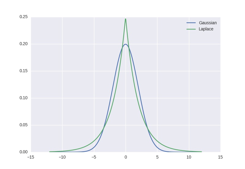
The fact that the Laplace exhibits high tails explains why the outliers do not have such a huge impact on the MLE obtained parameters, as having values off-centered is still probable. For the Gaussian case, it is so unlikely to have a value outside of +/- 6 sigmas that any outlier will have a tremendous influence on the MLE parameters. Hence the higher robustness of over .
There is nothing new research-wise in this post, robust norm was a hot topic in the 60s, for instance with the famous Huber loss, but I think this makes for a beautiful illustration of the robustness of the norm to outliers.
Recent Comments